
Bitemporal Modeling

A few articles ago, we wrote about data modeling and most recently about data warehousing using star schema for slowly changing dimension (SCD) Type 2. In this article, we continue our series on data modeling and data warehousing with a discussion of bitemporality, otherwise know as bitemporal modeling or bitemporal history.
A Thought Experiment
An article from dataversity has an instructional thought experiment that illustrates bitemporality:
“Imagine we have a payroll system that knows that an employee has a rate of $100/day starting on Jan. 1.
On Feb. 25, we run the payroll with this rate.
On March 15, we learn that, effective on Feb. 15, the employee’s rate changed to $211/day.
What should we answer when we are asked what the rate was for Feb. 25?”
The example above comes from Martin Fowler’s excellent blog post on bitemporal history.
SCD Type 1
If you use Type 1 slowly changing dimensions for your star schema based data warehouse, whenever a dimension record changes, the original record in the warehouse is updated.
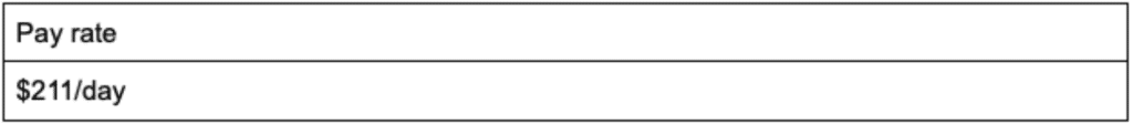
For the example above, on March 15, when we learned that the employee’s pay rate changed, effective Feb. 15, from $100/day to $211/day, we updated the dimension record for that employee.
Table as of March 14:
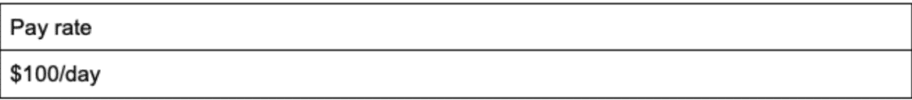
Table as of March 15:
For the payroll run that was completed on Feb. 25, the original pay rate record ($100/day) would have been used. However, if you rerun the payroll on a date after March 15, the payroll run would use the pay rate $211/day, which was updated on March 15 – so the payroll run executed after March 15 would give a different result than one run prior.
To calculate payroll correctly both of these data points are required – the original pay rate and the updated pay rate. Unfortunately, when using SCD Type 1, only a single data point is available.
If you run the payroll prior to March 15, the payroll will be wrong because it will use the incorrect pay rate for Feb. 15 and days afterward. If you run the payroll after March 15, the payroll will be wrong because it will use the incorrect pay rate for days prior to Feb. 15.
SCD Type 2
If you use Type 2 slowly changing dimensions for your star schema based data warehouse, whenever a dimension record changes, the original record remains in the warehouse and a new record is inserted with the corrected data. The original record is updated so that it is no longer the current record.
For the example above, on March 15, when we learned that the employee’s pay rate changed, effective Feb. 15, from $100/day to $211/day, we added a new dimension record for that employee and we updated the original record by setting its “end_date” value to the current date of March 15.
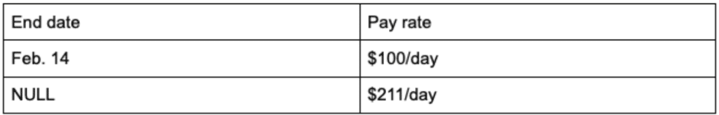
For the payroll run that was completed on Feb. 25, the original pay rate record ($100/day) would have been used. However, if you rerun the payroll on a date after March 15, the payroll run would use the pay rate $211/day, which was added on March 15 – so the payroll run executed after March 15 would give a different result than one run prior.
With SCD Type 2, previous records remain in the database, so it is possible to look back at them. Processes such as payroll runs, in order to consider back-dated changes, would query for multiple records for the payroll period being calculated. For our example, assuming we are calculating payroll for the period of Feb. 1 – Feb. 25, we would need to return: 1. The current pay rate records; 2. All pay rate records with end dates within our payroll period of Feb. 1 – Feb. 25. The records returned would, at least theoretically, allow you to calculate payroll correctly.
Even though we save historical pay rate records, we can still have problems because the “end_date” field on our dimension records only provides insight into what the pay rate was on certain dates. It does not tell us what records our payroll run actually used for its calculation, because it provides no information about when the records were added to the system.
From our example, we know that the new pay rate, though it was effective Feb. 15, was only added to the system on March 15. So if our payroll run occurred before March 15, it would have only known about the $100/day pay rate record, so would have calculated based on that rate. If the employee in question complains that they were underpaid, if we look back at our records on a date after March 15, the records would appear to be correct.
Bitemporality can help resolve this issue by saving a separate timeline, in addition to the record validity timeline, which is the timeline for the existence of the records themselves. For example:
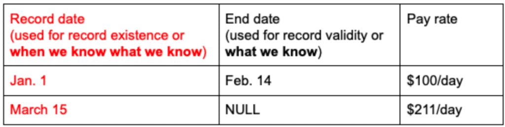
The second timeline for each record is the essence of bitemporality and it allows us to determine not just what a value was on a given date but also when we knew that value. For our example, we can answer the question of what the pay rate was on Feb. 25 as we knew it on Feb. 25; as we knew it on March 15; etc. This allows us to say both what we knew to be true and when we knew it to be true.
Summary
As you can see, bitemporality can be difficult to reason about and requires careful thought to design solutions correctly. Even given this added complexity, for cases where back-dated changes are possible, bitemporality enables you to design solutions that will allow you to answer questions accurately.
Up next
Common problems with star schema modeling.